Transformation and Rotation matrices
Table of contents
Intro
The transformation matrix is a much wider concept but for orientation in 3D space, we will restrict it into a rotation matrix. So transformation matrix transforms (wow) any vector from one reference frame into the other:
\[\begin{gather} \mathbf{v}^{(0)}=\mathbf{R}_{1}^{0}\mathbf{v}^{(1)} \end{gather}\]Rotation matrix rotates any vector about a specific axis and about a set angle (in this example rotation of vector $\mathbf{v}=\left[\begin{array}{ccc} 1,1,1\end{array}\right]^T$ about $90^{\circ}$ in Z-axis):
\[\begin{gather}\mathbf{v'=\mathbf{R}_z(90^{\circ})\mathbf{v}}=\left[\begin{array}{ccc} 0 & -1 & 0\\ 1 & 0 & 0\\ 0 & 0 & 1 \end{array}\right] \left[\begin{array}{c}1\\1\\1 \end{array}\right]= \left[\begin{array}{c} -1\\ 1\\ 1 \end{array}\right] \end{gather}\]Rotation and Transformation
It is important to see the difference between the transformation of a vector between reference frames and the rotation of a vector. These two are related to each other but not the same.
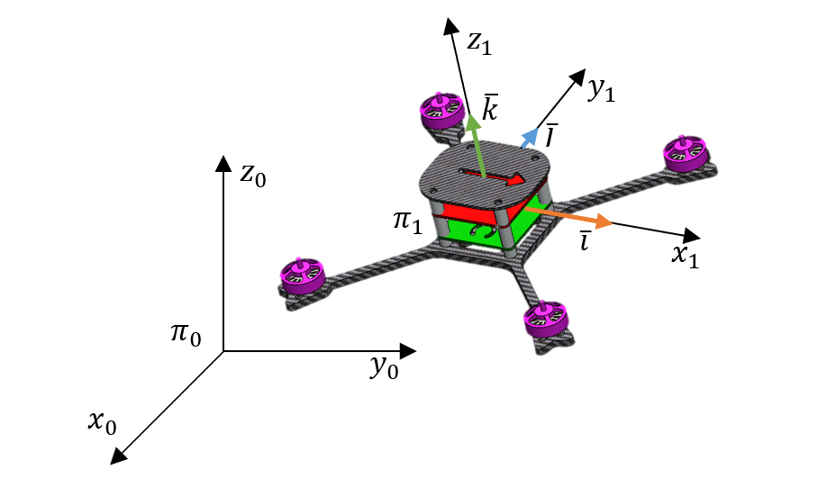
Assuming that a certain reference system ($\pi_1$) is associated with the object, and on each of its axes there are versors (see picture below); additionally, there is a fixed reference system associated with the static environment ($\pi_0$). The transformation matrix from the object-related system ($\pi_1$) to the global system ($\pi_0$) will be equal to the notation of 3 versors, associated with the moving system, in the global frame (\ref{eq:transformation matrix}).
Due to the orthogonality of this matrix, its inverse is equal to its transposition:
\[\begin{gather}\mathbf{R}_{1}^{0}\mathbf{R}_{0}^{1}= \mathbf{I}\Rightarrow (\mathbf{R}_{1}^{0})^{-1}=\mathbf{R}_{0}^{1}=(\mathbf{R}_{1}^{0})^{T} \end{gather}\]The transformation matrix defines explicitly the orientation and in a very simple way allows to perform the transformation of vectors from one system to another. It is also quite intuitive. Unfortunately, due to numerical inaccuracies, it quickly happens that the matrix is not normalized (loses orthonormality) and it is necessary to normalize it, which is a rather computationally expensive process.
Euler angles can be easily extracted from the transformation matrix. This can be seen very well when one writes the transformation matrix in 3D space as a complex of 3 basic rotations (rotations about 3 principal axes of the global system). For the rotation scheme $Z^{(0)}-Y^{(1)}-X^{(2)}$ (used for the drone) it looks as follows:
\[\begin{gather}\mathbf{R}_{1}^0=\mathbf{R}_z(yaw)\mathbf{R}_y(pitch)\mathbf{R}_x(roll)=\label{eq:euler angle to R}\\ \nonumber\\ \left| \mathbf{R}_z(\gamma)= \left[ \begin{array}{ccc} \cos{\gamma} & -\sin{\gamma} & 0 \\ \sin{\gamma} & \cos{\gamma} & 0 \\ 0 & 0 & 1 \end{array} \right] \mathbf{R}_y(\beta)=\left[\begin{array}{ccc} \cos{\beta} & 0 & \sin{\beta} \\ 0 & 1 & 0 \\ -\sin{\beta} & 0 & \cos{\beta} \end{array} \right] \mathbf{R}_x(\alpha)= \left[ \begin{array}{ccc} 1 & 0 & 0 \\ 0 & \cos{\alpha} & -\sin{\alpha} \\ 0 & \sin{\alpha} & \cos{\alpha} \end{array} \right] \right| \nonumber\\ \nonumber\\ =\left[ \begin{array}{ccc} \cos{\gamma}\cos{\beta} & \cos{\gamma}\sin{\beta}\sin{\alpha}-\sin{\gamma}\cos{\alpha} & \cos{\gamma}\sin{\beta}\cos{\alpha}+\sin{\gamma}\sin{\alpha}\\ \sin{\gamma}\cos{\beta} & \sin{\gamma}\sin{\beta}\sin{\alpha}+\cos{\gamma}\cos{\alpha} &\sin{\gamma}\sin{\beta}\cos{\alpha}-\cos{\gamma}\sin{\alpha} \\ -\sin{\beta} & \cos{\beta}\sin{\alpha} & \cos{\beta}\cos{\alpha} \end{array} \right] \label{eq:transformation matrix 3D} \end{gather}\]Euler angles from transformation matrix
From matrix (\ref{eq:transformation matrix 3D}) Euler angles can be easily extracted:
\[\begin{align} \gamma&=atan2(R_{21},R_{11})\label{eq:matrix trans to yaw}\\ \beta&=\arcsin{(-R_{31})}\\ \alpha&=atan2(R_{32},R_{33})\label{eq:matrix trans to roll} \end{align}\]You can see here exactly the problem of determining the Euler angles in the surrounding of the singular point ($\beta \rightarrow \pm \frac{\pi}{2}$). It is worth noting that for different conventions of Euler angles the formulas binding the transformation matrix and these angles (\ref{eq:matrix trans to yaw})-(\ref{eq:matrix trans to roll}) will have a different form, but the numerical value of the matrix (\ref{eq:transformation matrix 3D}) will be the same.