Quaternion derivative
Table of contents
Intro
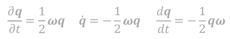
When I was searching for uses of quaternions in orientation algorithms, there was always one equation that was shown with no explanation:
\[\begin{gather}\dot{\mathbf{q}}(t)=\frac{1}{2}\boldsymbol{\omega}\mathbf{q}(t) \end{gather}\]but sometimes it was:
\[\begin{gather}\dot{\mathbf{q}}(t)=-\frac{1}{2}\boldsymbol{\omega}\mathbf{q}(t) \end{gather}\]or
\[\begin{gather}\dot{\mathbf{q}}(t)=-\frac{1}{2}\mathbf{q}(t) \boldsymbol{\omega}\end{gather}\]Moreover, when I was looking for any derivation of these formulas I found out that all resources were several pages - not very encouraging for me or derivations were not complete in their calculations, which was even more frustrating when you were thinking that finally, you would understand this.
So, I decided to do it myself in 2 ways: based on quaternion interpretation and old-fashioned derivative from the definition. Also, I will discuss frames of reference in which all of the elements are presented. I will provide some transformations of an equation in which everything will be well described and you will be able to better understand equations used in many other resources. I highly recommend reading an Introduction to quaternions and Quaternions as rotations because although derivatives are based on knowledge from basic calculus some of the properties of quaternions and their interpretation are needed to fully understand these calculations.
Option I: From the definition
Let’s start with the traditional derivate from the definition of derivative:
\[\begin{gather} \dot{\mathbf{q}}(t)=\lim_{\Delta t\to 0} \frac{\mathbf{q}(t+\Delta t)-\mathbf{q}(t)}{\Delta t}\\ \nonumber\\ \mathbf{q}(t)=\cos{\left(\frac{\omega}{2}t\right)}+\mathbf{v}\sin{\left(\frac{\omega}{2}t\right)}=\nonumber\\ =\cos{\left(\frac{\theta(t)}{2}\right)}+\mathbf{v}\sin{\left(\frac{\theta(t)}{2}\right)}\\ \nonumber\\ \mathbf{q}(t+\Delta t)=\mathbf{q}(\Delta t)\mathbf{q}(t)=\nonumber\\=\left[\cos{\left( \frac{\omega}{2}\Delta t\right)}+\mathbf{v}\sin{\left(\frac{\omega}{2}\Delta t\right)}\right]\left[\cos{\left(\frac{\omega}{2}t\right)}+\mathbf{v}\sin{\left(\frac{\omega}{2}t\right)}\right]\\ \nonumber\\ \dot{\mathbf{q}}(t)=\lim_{\Delta t\to 0} \frac{(\mathbf{q}(\Delta t)-1)\mathbf{q}(t)}{\Delta t} \end{gather}\]by using the approximations: \(\lim_{\Delta x\to 0}\cos{(\Delta x)}=1,\ \lim_{\Delta x\to 0}\sin{(\Delta x)}=\Delta x\):
\[\begin{gather} \dot{\mathbf{q}}(t) =\lim_{\Delta t\to 0} \frac{\left(1+ \mathbf{v}\frac{\omega}{2}\Delta t-1\right)\mathbf{q}(t)}{\Delta t}=\nonumber\\=\lim_{\Delta t\to 0} \frac{\mathbf{v}\frac{\omega}{2}\Delta t}{\Delta t}\mathbf{q}(t) =\frac{1}{2}\boldsymbol{\omega}\mathbf{q}(t) \end{gather}\]Option II: Natural interpretation
Now, let’s see a more pleasant way to obtain a derivate - based on the interpretation of quaternions as rotations. The quaternion describing the rotation from the initial position to the current position can be written as:
\[\begin{gather} \mathbf{q}(t)=\mathbf{q}_{\omega}^t\mathbf{q}_0 \end{gather}\]Next, assuming constancy of angular velocity $\boldsymbol{\omega}=const.$ We can use an exponential form of quaternion and write:
\[\begin{gather} \mathbf{q}_{\omega}=\cos{\frac{\omega}{2}} + \mathbf{v}\sin{\frac{\omega}{2}}\\ \nonumber\\ \mathbf{q}_{\omega}^t=e^{\mathbf{v}\frac{\omega}{2}t}\\ \nonumber\\ \dot{\mathbf{q}}(t)=\frac{d}{dt}(\mathbf{q}_{\omega}^t\mathbf{q}_0)=\frac{d}{dt}\left(\mathbf{q}_{\omega}^t\right)\mathbf{q}_0+\mathbf{q}_{\omega}^t\frac{d}{dt}\mathbf{q}_0=e^{\mathbf{v}\frac{\omega}{2}t}\mathbf{v}\frac{\omega}{2}\mathbf{q}_0\end{gather}\]from direct calculations, it can be shown that:
\[\begin{gather} e^{\mathbf{v}\frac{\omega}{2}t}\mathbf{v}\frac{\omega}{2}=\mathbf{v}\frac{\omega}{2}e^{\mathbf{v}\frac{\omega}{2}t} \end{gather}\]In general multiplication (of quaternions) is not commutative. See the end of this post for an explanation.
additionally $\mathbf{v}\omega$ = $\boldsymbol{\omega}$ so:
\[\begin{gather} \dot{\mathbf{q}}(t)=\frac{\boldsymbol{\omega}}{2}e^{\mathbf{v}\frac{\omega}{2}t}\mathbf{q}_{0}=\frac{1}{2}\boldsymbol{\omega}\mathbf{q}(t) \end{gather}\]The importance of the reference frame
The above formulas for the derivative of the quaternion of rotation use the quaternion q which is the quaternion transforming from the drone-related system to the global frame. However, the quaternion describing the transformation from the global system to the local system is more commonly used. We know that:
\[\begin{gather} {}^{b}_{g}\mathbf{q}={}^{g}_{b}=\mathbf{q}^{-1}={}^{g}_{b}\mathbf{q}^{*} \end{gather}\]analogically derivative:
\[\begin{gather} {}^{b}_{g}\dot{\mathbf{q}}={}^{g}_{b}\dot{\mathbf{q}}^{*} \end{gather}\]using a formula for conjugation of quaternions multiplication:
\[\begin{gather} {}^{b}_{g}\dot{\mathbf{q}}=\left( \frac{1}{2}\boldsymbol{\omega}{}^{g}_{b}\mathbf{q}(t)\right)^{*}=\frac{1}{2} {}^{g}_{b}\mathbf{q}(t)^{*}\boldsymbol{\omega}^{*}=-\frac{1}{2}{}^{b}_{g}\mathbf{q}(t)\boldsymbol{\omega} \end{gather}\]Note, that the $\boldsymbol{\omega}$ which was used in the above formulas is a vector in the global system. We were considering quaternions which describe global rotation from default orientation to end one. The measurements of the gyroscope are taken in the local frame. Taking this into account, it can be written:
\[\begin{gather} \begin{split} {}^{b}_{g}\dot{\mathbf{q}}=-\frac{1}{2}{ {}^{b}_{g}\mathbf{q}(t)\boldsymbol{\omega}^{(g)}}=-\frac{1}{2}{ {}^{b}_{g}\mathbf{q}(t)\left( {}^{g}_{b}\mathbf{q}(t)\boldsymbol{\omega}^{(b)} {}^{g}_{b}\mathbf{q}(t)^{*}\right)}=\\ =-\frac{1}{2} {}^{b}_{g}\mathbf{q}(t) {}^{g}_{b}\mathbf{q}(t)\boldsymbol{\omega}^{(b)} {}^{b}_{g}\mathbf{q}(t)=-\frac{1}{2}\boldsymbol{\omega}^{(b)} {}^{b}_{g}\mathbf{q}(t) \end{split} \end{gather}\]So, this is the final equation:
\[\begin{gather} {}^{b}_{g}\dot{\mathbf{q}}=-\frac{1}{2}\boldsymbol{\omega}^{(b)} {}^{b}_{g}\mathbf{q}(t) \label{eq:derivative of quaternion} \end{gather}\]It takes gyroscope measurements in the local frame (drone frame) and quaternion that describes the transformation from the global frame to the local frame. If you want to use the same quaternion but measurements are in the global frame you need to use:
\[\begin{gather} {}^{b}_{g}\dot{\mathbf{q}}=\frac{1}{2} {}^{b}_{g}\mathbf{q}(t)\boldsymbol{\omega}^{(g)} \end{gather}\]If you have the measurements in the global frame and quaternion describing the rotation from the global to the local frame you can use the:
\[\begin{gather} {}^{g}_{b}\dot{\mathbf{q}}=\frac{1}{2}\boldsymbol{\omega}^{(g)} {}^{g}_{b}\mathbf{q}(t) \end{gather}\]So, as you can see it is important to know what reference frame you’re using and which quaternion is used but now you should be able to transform these equations if necessary, at least it is my hope.
Why $e^{\mathbf{v}\frac{\omega}{2}t}\mathbf{v}\frac{\omega}{2}=\mathbf{v}\frac{\omega}{2}e^{\mathbf{v}\frac{\omega}{2}t} $ is correct?
So, if we decompose the formulas into the same forms:
\[\begin{gather} L:\ e^{\mathbf{v}\frac{\omega}{2}t}\mathbf{v}\frac{\omega}{2}= (\cos{\frac{\omega}{2} t}+\mathbf{v}sin{\frac{\omega}{2} t})(0+\mathbf{v}\frac{\omega}{2})\\ \nonumber \\R:\ \mathbf{v}\frac{\omega}{2}e^{\mathbf{v}\frac{\omega}{2}t}= (0+\mathbf{v}\frac{\omega}{2})(\cos{\frac{\omega}{2} t}+\mathbf{v}sin{\frac{\omega}{2} t}) \end{gather}\]it is important that only vector $\mathbf{v}$ has imaginary symbols and the rest of the components can be written as some scalars:
\[\begin{gather} L:\ (\alpha_1+\mathbf{v}\beta_1)(\alpha_2+\mathbf{v}\beta_2)\\ \nonumber \\R:\ (\alpha_2+\mathbf{v}\beta_2)(\alpha_1+\mathbf{v}\beta_1) \end{gather}\]now we can perform multiplication:
\[\begin{gather} L:\ \alpha_1\alpha_2+\alpha_1\mathbf{v}\beta_2 +\mathbf{v}\beta_1 \alpha_2+\mathbf{v}\beta_1\mathbf{v}\beta_2\\ \nonumber \\R:\ \alpha_2\alpha_1+\alpha_2\mathbf{v}\beta_1+\mathbf{v}\beta_2\alpha_1+\mathbf{v}\beta_2\mathbf{v}\beta_1 \end{gather}\]rearranging components we can show that $L=R$:
\[\begin{gather} L:\ \alpha_1\alpha_2+\mathbf{v}(\alpha_1\beta_2 +\beta_1 \alpha_2)+\mathbf{v}\mathbf{v}\beta_1\beta_2\\ \nonumber \\R:\ \alpha_2\alpha_1+\mathbf{v}(\alpha_2\beta_1+\beta_2\alpha_1)+\mathbf{v}\mathbf{v}\beta_2\beta_1 \end{gather}\]